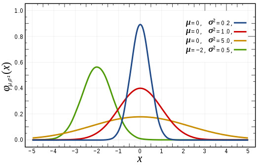
It turns out that normally distributed values are quite important in statistics. Not only because the pattern is remarkably common, the central limit theorem enables statisticians to infer conclusions about how a given treatment will affect a given population. To make such inferences, we need to learn about the Probability Density Function and a useful shortcut: the Z Table.
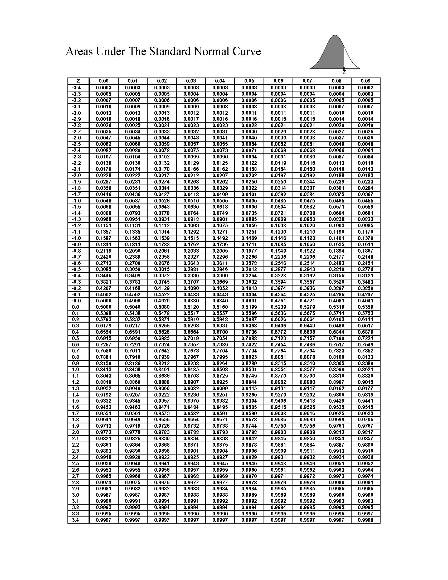
In a normally distributed population of values, a few things are true. First, the distribution is symmetrical and the mean median and mode are all equivalent. Due to these factors, we know that more than half of the observations will fall within one standard deviation (σ) of the mean (μ), and the vast majority fall within 2 standard deviations. More exacting percentages of observations which fall within a given range can be calculated using a continuous probability density function (PDF), or one can look up those numbers on a z-table which lays out a pre-calculated portion of the range of the PDF for a normal distribution.
To demonstrate the usage of a probably density function and z-table took up, let’s look a fictional sample of human height (both male and female).
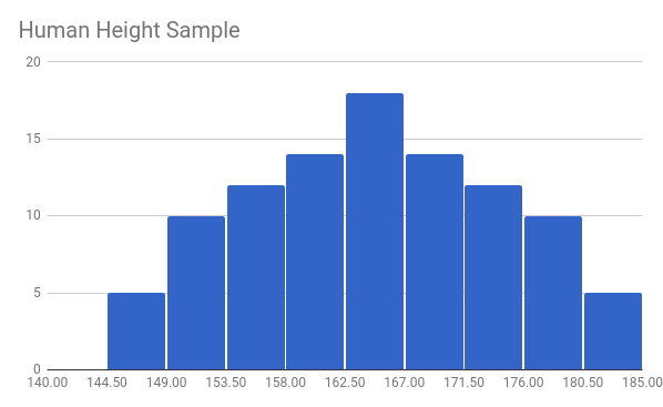
This sample – as would a real sample of human height – is normally distributed with a mean of 164.5 cm (the real averages according to Wikipedia are 175.7 cm and 161.8 cm for men and women respectively) and a standard deviation of 9.7 cm. Our distribution curve would look like something like this:
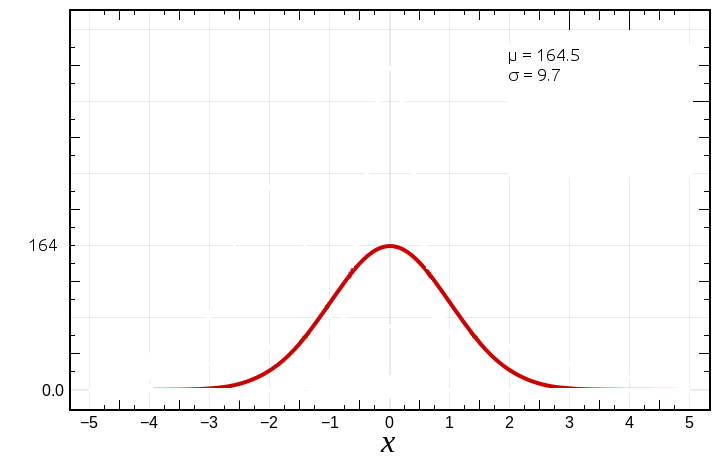
On the graph, we’ve normalized our data with z values on the x axis. Z values zero out at the mean μ. A value of 1 is μ+1 standard deviation from the mean; in this case, 164.5 + 1σ = 164.5 + 9.7 = 174.2. A z value of -1 is μ-1 standard deviation from the mean, or 164.5 – 1σ = 164.5 – 9.7 = 154.8.
We know, since in a normal distribution mean = median = mode; and that half the values fall before the median and half after, that if a person in the measured population’s height were 164.5 cm – i.e. median height – then half the people measured would be taller and half short then them. But what if a person was 174.2 cm tall? How many people would be taller than that person? Well, we can look that up on our z-table (link to z-table above). Just go to the 1.0 row and look in the first (i.e. 0.00) column.

Since probability is always a number between 0 (impossible) and 1 (absolutely certain) we can see that the 174.2 cm tall person is taller than ~84% of the rest of the group. Conversely, ~16% of group members are taller than this person. We can calculate a z value for any person in the group with the following formula:
# let x be the observed height.

z = (x - μ)/σ
Once we have the z value, we can determine what percentile the observation fall into. Using this formula, we can also calculate the likelihood a person falls within a range as well.